Phase (Un)Wrapping
In this article we explain the cause of phase wrapping in indirect Time-of-Flight (iToF) depth cameras, the measurement error it creates, and the different methods of resolving the measurement error to enable longer distance measurements.
What is Phase Wrapping?
Indirect Time-of-Flight (iToF) depth cameras measure the phase difference between an emitted laser pulse and its reflection. This phase difference encodes how far the light has travelled and thus how far away the object is, and the phase measurement is done for every pixel simultaneously.
The depth measurement is performed by correlating the reflected laser pulse with a reference signal. Both of these signals are square waves, and the correlated signal is a triangular wave, as animated below.
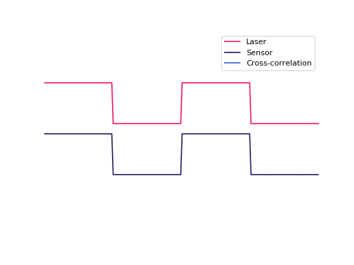
The phase of the triangular wave encodes the distance travelled, where the phase is between \(0\) and \(2\pi\). From the phase we can calculate the distance, using the equation below, where \(\phi\) is the phase, \(c\) is the speed of light, and \(f\) is the square wave modulation frequency.
$$ d = \frac{\phi}{2\pi} \frac{c}{2f} $$
The phase is normalized by \(2\pi\), and multiplied by a constant, the speed of light over two times the modulation frequency. The extra factor of 2 comes in because the light has travelled to the object and back, doubling the distance we are interested in measuring. When the phase is \(2\pi\), the maximum distance that can be measured is
$$ d_{max} = \frac{c}{2f} $$
Current iToF image sensors, like the Melexis MLX75027, have a modulation frequency range of 10–100MHz which corresponds to a maximum distance of 15m to 1.5m.
Phase measurement is circular, meaning when the measurement goes past \(2\pi\) the measurement goes back to 0 (this is called phase wrapping), because the measurement has moved onto the next repetition, in our case the next triangular peak from figure 1. The animation below plots the actual distance verse the measure phase for 40MHz.
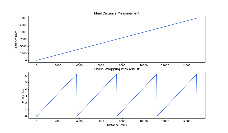
Due to phase wrapping, an object will always be measured in the first distance interval, called ambiguity intervals, as shown in Figure 3. It is possible for the object to be located in any of the ambiguity brackets, and the purpose of phase unwrapping is to figure out which bracket is the correct one.
![Figure 3: Graphical representation of phase wrapping. Objects beyond the maximum distance are phase wrapped into the first ambiguity bracket, when their actual location could be in any of the brackets. This figure was Inspired by [1]](/images/phase-wrapping/phase-wrapping.webp)
Phase Unwrapping
There are three different approaches to calculating the correct distance. The first is to operate the camera at a suitable modulation frequency such that phase wrapping is unlikely to occur, this is the most basic approach. The second approach is to use measurements at multiple modulation frequencies, and the third approach is to use spatial information in the image to predict the correct distance.
Lower the Frequency
The easiest approach is to lower the modulation frequency until phase wrapping is not going to cause issues as there is no signal returning from objects further away than the first ambiguity bracket.
This this decreases measurement precision, as the phase noise is constant* between frequencies, so the same phase noise at a lower frequency results in a higher distance noise. This is the a major motivating factor to use higher modulation frequencies.
Multi-frequency Approaches
These approaches measure two or more frequencies for each pixel to phase unwrap the measurement. These methods build upon phase unwrapping methods from interferometry. Payne et. al [2] suggested using two frequencies for phase unwrapping and points out the advantage of using higher modulation frequencies.
The new maximum distance is determined by greatest common denominator between the two modulation frequencies, so the new effective frequency is
$$ f_{amb} = gcd(f_1, f_2) $$
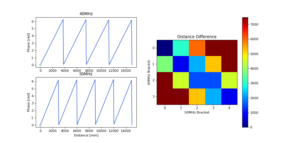
For the two frequencies 40MHz and 50MHz the greatest common denominator is 10MHz, and 10MHz has a maximum distance of 15m, compared to 3m for 50MHz and 4.5m for 40MHz.
Brute Force It!
The idea is that for two frequency measurements there is a single distance that “makes sense” (minimizes the error) of the two measurements. The unwrapped phases (theta) can be written as
$$ \theta_{f1} = \phi_{f1} + 2\pi k $$ $$ \theta_{f2} = \phi_{f2} + 2\pi l $$
Where \(k\) and \(l\) are integers, we want to select them to minimize the distance difference, as this equation equals zero in the noiseless case
$$ \frac{\theta_{f1}}{2\pi} \frac{c}{2f_1} - \frac{\theta_{f2}}{2\pi} \frac{c}{2f_2} = 0 $$
The brute force search is visualized in the animation below, where we calculate every possible l and k value and compute the distance difference and find the minimum. The location of the minimum gives which l and k values to use that correctly phase unwraps the measurement.
The above method is the naïve (brute force) approach, as it searches over all possible l and k values. A more optimal algorithm is the Chinese remainder theorem [1]. There are a few numerical improvements to speed up the search, such as only computing the most likely indexes. Adrian Jongenelen worked on phase unwrapping as part of his PhD thesis [1] and implemented a real time processing method on an FPGA.
Another alternative to the Chinese remainder theorem is to only search over the subset of indices that are possible. For the 40,50MHz pair about that would be k, and l values of (0,0),(0,1),(1,1),(1,2),(2,2),(2,3),(3,3), and (3,4), so the search is over 8 pairs instead of the possible 20 pairs.
The video below demonstrates phase unwrapping using a Chronoptics Kea indirect time-of-flight camera capturing two modulation frequencies, 80MHz and 100MHz. This video shows phase unwrapping in action, taking two modulation frequencies, 60 and 80 MHz and combining them together to extend the maximum distance.
The Microsoft Way
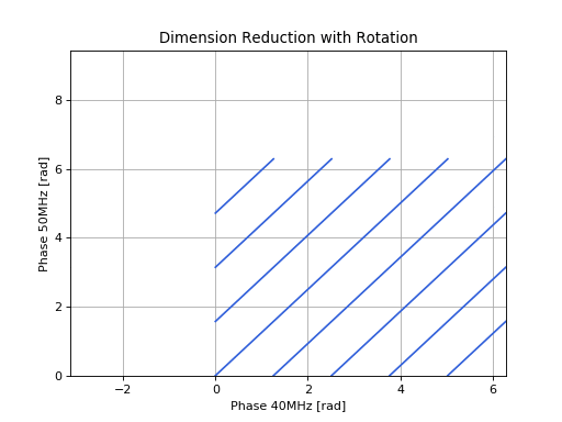
Microsoft filed for a patent for multi-frequency phase unwrapping [3], developed by Benedetti et al. This approach starts by the observation that plotting the measured phase of one frequency against the phase of a second frequency results in lines on that surface. Measurements should only ever land on these lines, and which line the measurement lands on represents the distance offset (ambiguity bracket) so we can phase unwrap the measurement.
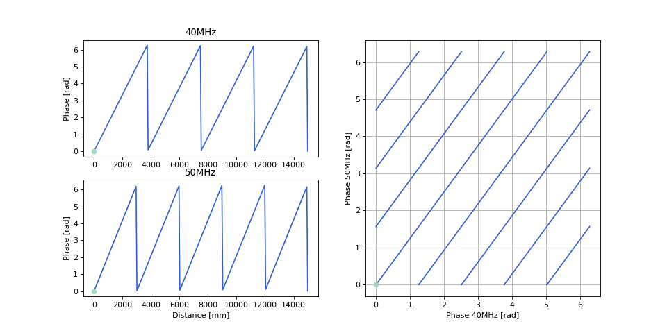
The second observation is that dimension reduction is possible, by rotating the lines so they collapse into a set of points. The closest point to a measurement encodes the ambiguity bracket. This approach can be expanded to multiple modulation frequencies, for example 3 frequencies.
For three frequencies the lines on a plane become lines in 3D space from adding the extra dimension. The rotation then reduces the dimension to points on a 2D plane. The maximum distance is still set by the greatest common denominator (GCD), so for frequencies [75MHz,90MHz,120MHz] the GCD is 15MHz, resulting in a maximum distance of 10m.
Other Ways
Droeschel et. al [4] used a mixture of frequencies and spatial information for phase unwrapping, as the two frequencies available were 29MHz and 31MHz. The spatial information was looking for pixels that jumped distance by \(2\pi\).
Lawin et. al [5] used the frequency information with the amplitude and spatial (neighboring pixels) for more robust phase unwrapping, removing the “salt and pepper” noise present in per-pixel phase unwrapping in low signal conditions.
Single-Frequency Methods
Single frequency phase unwrapping methods attempt to unwrap the phase based on information contained in a single frequency measurement, using the spatial information provided by the image sensor. This is often similar to phase unwrapping techniques used for interferometric synthetic aperture radar.
The methods use the following ideas/constraints for phase unwrapping
- Jumps in distance that correspond to \(2\pi\) between pixels are most likely phase wrapping, and these jumps can be unwrapped.
- Object surfaces are smooth.
- The assumption of Lambertian surfaces, that the amplitude drops off by 1/d², therefore close dark objects are probably phase wrapped.
- In some scenes (like a hallway) we know the pixels at the bottom of the image are correctly measured so we can phase unwrap by following the gradient of distance down the hallway and phase unwrapping any pixel jumps that correspond to \(2\pi\).
Ryan Crabb’s PhD thesis [6] was on single frequency phase unwrapping for ToF depth sensing. Crabb developed two methods for single frame phase unwrapping and compared his results against Choe et. al [7].
McClure et. al [8] demonstrated a processing pipeline to phase unwrap with a single frame. McClure started by classifying pixels based on their amplitude data, as the amplitude of reflection drops away as 1/d², therefore lower amplitude pixels are more likely to be phase wrapped. Then with a filtering pipeline to segment out different objects in the scene the algorithm classified each object as phase wrapped or not.
The disadvantage of single frequency methods are that they can be fooled. They work well in some situations, such as using a ToF camera in a known use case, however they can be quick to break when presented with generalized scenes.
With advances in Machine Learning, I am sure there will be a paper on using deep learning to solve phase unwrapping on ToF cameras using a single frequency, that might generalize to a better solution. If you have written such a paper, or plan to, let me know! Currently the deep learning approach to ToF has been to replace the full depth pipeline with a neural network, such as DeepToF [9], of which part of the pipeline is phase unwrapping.
Conclusion
The best phase unwrapping method depends on your depth sensing application. When the number of frames is required to be low and there is limited computational power then decreasing the modulation frequency is best. When more frames can be acquired the multi-frequency methods become possible. With theses solutions the computation per-pixel is low, and the result is deterministic. In the case where a small number of frames is required, computation power available, and there are some predictable scene constraints then single frequency methods are appropriate. The best approach depends on the application which determines the power budget, frames per second, computational complexity, and accuracy.
References
[1] Jongenelen, A. P. P. (2011). Development of a compact, configurable, real-time range imaging system.
[2] Payne, A. D., Jongenelen, A. P., Dorrington, A. A., Cree, M. J., & Carnegie, D. A. (2009). Multiple frequency range imaging to remove measurement ambiguity. In Optical 3-d measurement techniques.
[3] Benedetti, A., Perry, T., Fenton, M., & Mogallapu, V. (2014). U.S. Patent Application №13/586,391.
[4] Droeschel, D., Holz, D., & Behnke, S. (2010, October). Multi-frequency phase unwrapping for time-of-flight cameras. In 2010 IEEE/RSJ International Conference on Intelligent Robots and Systems (pp. 1463–1469). IEEE.
[5] Lawin, F. J., Forssén, P. E., & Ovrén, H. (2016, October). Efficient multi-frequency phase unwrapping using kernel density estimation. In European Conference on Computer Vision (pp. 170–185). Springer, Cham.
[6] Crabb, R. E. (2015). Fast Time-of-Flight Phase Unwrapping and Scene Segmentation Using Data Driven Scene Priors (Doctoral dissertation, UC Santa Cruz).
[7] Choi, O., Lim, H., Kang, B., Kim, Y. S., Lee, K., Kim, J. D., & Kim, C. Y. (2010, September). Range unfolding for time-of-flight depth cameras. In 2010 IEEE International Conference on Image Processing (pp. 4189–4192). IEEE.
[8] McClure, S. H., Cree, M. J., Dorrington, A. A., & Payne, A. D. (2010, January). Resolving depth-measurement ambiguity with commercially available range imaging cameras. In Image Processing: Machine Vision Applications III (Vol. 7538, p. 75380K). International Society for Optics and Photonics.
[9] Marco, J., Hernandez, Q., Munoz, A., Dong, Y., Jarabo, A., Kim, M. H., … & Gutierrez, D. (2017). DeepToF: off-the-shelf real-time correction of multipath interference in time-of-flight imaging. ACM Transactions on Graphics (ToG), 36(6), 1–12.
Notes
All these numbers have used the speed of light as 3e8, which is not quite right, but makes the maximum distance a round number.
The noise with modulation in theory should stay constant but doesn’t, as the illumination power changes, the demodulation contrast changes, and normally the temperature varies as well.